
Post Hoc Statistical Procedures
Post Hoc Statistical Procedures
Correlation and Regression
![]()
Overview
Analysis of covariance (ANCOVA) answers the question: What are the differences in the posttest scores if I hold constant the pretest scores? It is a procedure, like blocking and matching, that can be used to control for differences in pretest scores. ANCOVA can be used in either experimental or quasi-experimental designs.
The procedures used in blocking and matching are very mechanical. You go to your data file and select participants who have the same range of pretest scores (blocking) or you find a pairs of participants who have the same pretest score (matching). ANCOVA is a statistical model. It computes the regression equation between pretest and posttest scores for each group in the design and then uses the information from those regressions to answer the question pose above.
Before we get to the ANCOVA model we need to have an understanding of the concepts of correlation and regression.
Correlation
The conceptual formula
A correlation coefficient, r, is a measure of the relationship between two variables.
The Pearson product-moment correlation is defined the average of the sum of the cross-products of z-scores.
|
Where zx and zy are z scorers, and n = the number of pairs of data |
To use this formula you would first convert the scores within each variable to z-scores (this could be done with the descriptives procedure in SPSS). Find the product of the z-scores by multiplying each of the pairs of z-scores (zxzy). Then sum the products (S zxzy). Finally, divide the sum of the products by the number of scores (n) to find the correlation coefficient, r.
|
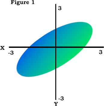
Recall that z scores have a mean of zero. About 99% of scores will fall between -3.00 and +3.00. The product of the z scores will be positive if both scores have the same sign, the product will be negative if the the two z scores have the opposite sign. Figure 1 shows a scatterplot of z-scores for two variables that are positively correlated. There are two quadrants where the products of the z scores will be positive, the lower-left quadrant (-zx*-zy) and the upper-right quadrant (+zx*+zy). Because the preponderance of the scores fall into those two quadrants the sum of the cross products will be positive and hence the correlation coefficient for those scores will be positive. |
|
|
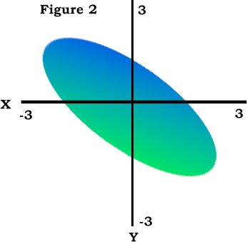
Figure 2 shows a scatterplot of z scores for two variables that are negatively correlated. There are two quadrants where the products of z scores will be negative, the upper-left quadrant (-zx*+zy) and the lower-right quadrant (+zx*-zy). Because the preponderance of the scores in Figure 2 fall into those two quadrants the sum of the cross products will be negative, and hence the correlation coefficient for those scores will be negative. |
|
|
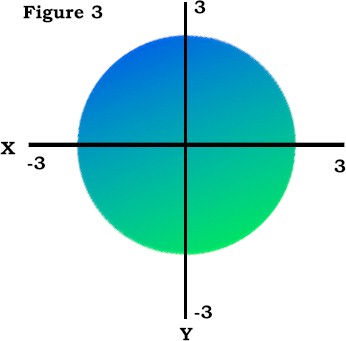
Figure 3 shows a scatterplot of z scores for two variables that are uncorrelated. The scores fall into all quadrants about equally, therefore the sum of the crossproducts will be near zero and the correlation coefficient will be near zero. |
|
The value of a Pearson product-moment correlation coefficient ranges from -1.00 through zero to +1.00. Positive values of r indicate that as values of one variable increase the values of the other variable also increase. Negative values of r indicate that as the values of one variable increase the values of the other variable decrease. The larger the absolute value of the correlation coefficient the greater the relationship between the two variables.
A computational formula
The z-score formula for a correlation is useful for conceptualizing a correlation, but you typically compute a correlation using raw scores rather than z scores. There are several different varieties of raw score formulas. The raw score formulas are all variations on formulas that transform the raw scores to z scores. The z score transformation involves subtracting a raw score from the mean and dividing by the standard deviation.
|
Where X is the raw score, M = the mean, and S = the standard deviation |
Here is a raw score formula for a correlation coefficient that uses the means and standard deviations of the two sets of raw scores.
|
Where XY = the crossproduct of the raw scores, MX and MY = the means of the two sets of scores, and SX and SY = the standard deviations of the two sets of scores. |
|
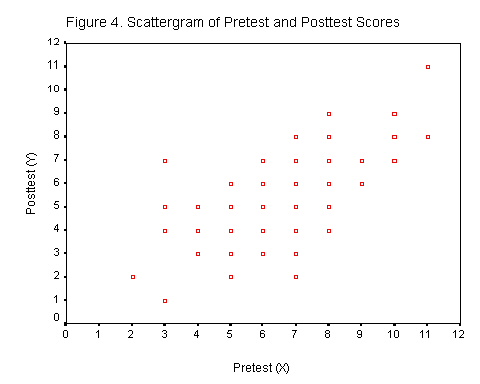
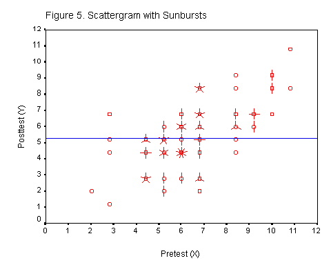
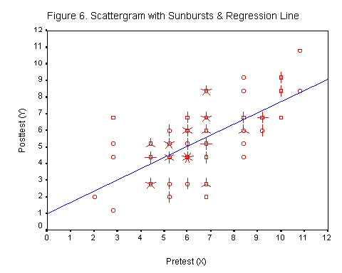
Lets apply this formula to a set of data. Figure 4 shows a raw score scatterplot for 100 cases. The scatterplot slopes upward to the right so the data are positively correlated. These data do not indicate multiple datapoints. Figure 5 includes "sunbursts," where each ray of the sunburst is one score. The horizontal line in Figure 5 is the mean of the posttest (Y) scores. |
|
|
Here is some relevant statistical information about these scores.
From that information you can compute r.
|
|
||||||||||||

Regression
Regression is used to predict one score from another. When talking about quasi-experimental designs we will want to predict the posttest score from the pretest score. The linear regression formula is
| Y' = a + byx X | Where Y' = the score to be predicted (the posttest score in this example), a is the intercept of the line, byx is the slope of the line, and X is a score on the pretest. |
This formula gives a line of best fit between X and Y.
Slope
The slope of the regression line is the amount of change in Y for a given change in X. A slope of .50 would indicate that for every 1.0 unit increase in X there is a corresponding .5 units increase in Y. The formula for the slope of the line, byx, is
The slope is found by multiplying the correlation between the two variables by the ratio of the standard deviations of Y and X. If the two standard deviations are equal to each other then the slope is the same as the correlation coefficient. (If you create a scatterplot from the z scores, then the slope of the regression line will be the correlation coefficient. Why?)
We have all the information we need to compute the slope.
![]()
We now have the slope of the line, we need to know where to place the line on the scatterplot. The intercept, a, tells us where to place the line with reference to the Y axis. The intercept is the point where the regression line crosses the Y-axis. It is the value of Y when X = 0.
Note that it is possible for the slope to be greater than or less than 1.00.
Intercept
The formula for the intercept is
| a = MY - bYXMX | Where My and MX are the means of Y and X respectively, and bYX is the slope. |
Plugging in the values that have already been computed, the value of the intercept is
a = MY - bYXMX
a = 5.28 - (0.68 * 6.32) = 0.98
The Regression Equation
The regression equation for this set of data is
Y' = a + byx X
Y' = 0.98 + 0.68X
|
By substituting values of X into the regression equation you can find the points to plot the regression line.
You can plot the regression line with the slope and the intercept. Or you can plot the regression line with any two points in the line. |
|
Interpretation
The values along the regression line are the predicted posttest scores, Y', for the corresponding pretest score, X. The regression line falls at the center of the scatterplot. It is the line of best fit for the scatterplot.
The distance between the predicted score, Y', and the obtained score, Y, is the amount of error in the prediction.
| Prediction error = Y - Y' |
The variance of the prediction errors is found by dividing the prediction error sums of squares by the number of cases.
|

The square root of the variance of the prediction errors is the standard deviation of the prediction errors. The standard deviation of the prediction errors has a special name in regression, it is the standard error of estimate.
|

The standard error of estimate is the standard deviation of the error scores. The standard error of estimate for this set of data is 1.42. That is, the standard deviation of the error scores around the regression line is 1.42
When it said that the regression line is the line of best fit, this means that the regression line minimizes the standard error of estimate. There is no other line through the scatterplot that has a smaller standard error of estimate.
When the correlation is zero
Consider the case where there is no correlation between X and Y. In this case the pretest scores would be of no help in predicting the posttest scores. The best estimate of the posttest scores would simply be the mean of those scores, see Figure 5. That is, the predicted posttest score would be the mean of those scores, Y' = MY.
|
||
| a = MY - bYXMX = MY - 0 = MY | ||
| Y' = a + byx X = MY |
What would be the error of prediction? It would be Y - MY. When the correlation is zero, then the variance of the prediction errors would be
|

This formula should look familiar to you, it is simply the variance of the scores. The square root of a variance is the standard deviation. We stated earlier that the standard deviation of the posttest scores, SY, was 1.89. So, if the correlation between the pretest and posttest scores was 0, then the standard error of prediction of the posttest scores would be 1.89.
If we just look at the posttest scores, without considering the pretest scores, then our standard error of estimate for the posttest scores is 1.89, which is the standard deviation of the posttest scores. When we take into account the correlation between the two sets of scores then the standard error of estimate is reduced from 1.89 to 1.42. Our estimates of the posttest scores are more precise. Our errors have decreased. We have increased the power of our prediction.
-03/15/99